

Executive Summary
We explore whether the latest generation of time series foundation models (TSFMs) can improve real-world energy forecasting. Using the highly volatile system imbalance (SI) of the Belgian electricity grid as a case study, we evaluate Chronos-2 in a realistic setting and benchmark it against a robust, well-established XGBoost model and a persistence baseline. Our findings show that Chronos-2 delivers strong zero-shot performance and clearly outperforms naive approaches, highlighting its value as a fast, low-effort starting point. However, it does not yet match the accuracy of a well-engineered and extensively validated model. In addition, applying TSFMs in practice still requires careful data preparation, validation, and integration into existing systems. Overall, while foundation models are rapidly closing the gap, they are not yet a plug-and-play replacement for specialized forecasting pipelines. Their strength today lies in rapid deployment and solid baseline performance, with clear potential as the technology continues to evolve.
Introduction
In this blog post, we put Chronos-2 to the test on a challenging real-world use case: forecasting the system imbalance (SI) of the Belgian electricity grid. Building on our previous blog series (From Volatility to Value: Outsmarting the Belgian System Imbalance and From Prototype to Production: The MLOps Backbone Behind Belgian System Imbalance Forecasting), we evaluate whether time-series foundation models (TSFMs) can deliver value in a realistic, operational energy setting.
Foundation models are gaining traction as a new paradigm in forecasting. They promise to simplify pipelines by reducing the need for extensive feature engineering, model tuning, and ongoing maintenance, potentially lowering infrastructure complexity. At the same time, even marginal improvements in forecast accuracy can have a direct financial impact on energy markets, enabling better asset steering and more informed trading decisions.
Yet, as adoption accelerates, so does skepticism. Some argue that the benefits of these models may be overstated, especially in complex, domain-specific settings. This raises a fundamental question: when put to the test in a real-world, high-stakes forecasting problem, do these models truly deliver on their promise?
The Next Generation of Time Series Foundation Models
The machine learning landscape has been reshaped by foundation models: large, pre-trained models capable of solving a wide range of tasks with minimal task-specific adaptation. This paradigm first emerged in natural language processing with models such as BERT and GPT, which demonstrated that a single model trained on large-scale data could be adapted to many downstream tasks. A similar shift followed in computer vision, with models such as Vision Transformers (ViTs) and CLIP enabling a wide range of visual tasks such as classification, retrieval, and zero-shot recognition within a single framework.
This idea, learning general representations from large and diverse datasets, has now started to extend to time series forecasting. As illustrated in Figure 1, the emergence of TSFMs has accelerated rapidly in recent years, with models such as Amazon’s Chronos-2 aiming to capture reusable temporal patterns across domains, rather than being trained for a single, narrowly defined task.
 Fig. 1: Release timeline of time series foundation models. The earliest model was introduced by Nixtla in October 2023, and the most recent release is Moirai-2 by Salesforce, launched in January 2026.
By learning from large-scale, heterogeneous collections of time series data, these models promise to generalize across different forecasting problems, potentially reducing the need for extensive feature engineering and model tuning. This raises a key question: can such models deliver meaningful value in real-world, high-stakes forecasting scenarios?
From Promise to Reality: What Time Series Foundation Models Need to Deliver
Traditionally, time series forecasting has relied on specialized statistical models such as ARIMA and its variants. While effective in controlled settings, these approaches struggle to incorporate rich contextual information such as weather signals, calendar effects, and market dynamics.
In practice, machine learning approaches such as gradient boosting models (e.g. XGBoost) and neural networks have demonstrated strong empirical performance when properly designed and tuned. However, achieving this performance typically requires substantial feature engineering, careful model tuning, and performance monitoring (e.g., retraining to mitigate performance drift) to adapt to changing system dynamics.
TSFMs aim to fundamentally change this paradigm. By pretraining on vast and diverse collections of time series data, they claim:
- Strong out-of-the-box performance, even without task-specific training (zero-shot forecasting)
- Native handling of covariates, reducing the need for manual feature engineering - unlike models such as XGBoost, which are not inherently designed for time series and therefore require explicit construction of temporal features (e.g., lags, leads, rolling statistics) to capture time dependencies
- Transferable temporal representations, enabling generalization across domains (cross-learning)
However, in a real-world energy setting, these claims need to be evaluated against practical requirements. In this blog post, we focus on the following questions:
- Performance: How does a TSFM compare to classical approaches, such as a well-tuned XGBoost model and a naive persistence baseline model?
- Operational complexity: What is required to run these models in production environments, including latency, scalability, and infrastructure overhead?
- Validation: How easy is it to evaluate on large historical datasets?
To answer these questions, we will focus deliberately on out-of-the-box performance. Instead of investing in fine-tuning or complex adaptations, we assess Chronos-2 in a realistic scenario by using it for SI forecasting.
While fine-tuning could further improve results, we treat this as future work. Our goal here is to provide a clear, honest assessment of what these models can deliver today, with minimal integration effort, and to frame the additional complexity required to unlock their full potential.
Chronos-2: A Universal Time Series Model
Given the rapid emergence of TSFMs, a natural question is which models are actually worth evaluating in a real-world setting. At ML6, we selected Chronos-2 as a candidate for experimentation based on its strong empirical performance, particularly on energy-related forecasting benchmarks.
As shown in Figure 2, Chronos-2 ranks as the top-performing model on the FEV-Bench energy domain leaderboard, which evaluates forecasting performance across 26 energy tasks. Performance is measured using two complementary metrics: skill score, which quantifies a model's relative improvement over a baseline (with higher values indicating better accuracy), and average win rate, which reflects how often a model outperforms competing approaches across tasks. Chronos-2 achieves strong results on both metrics, making it a relevant and credible choice for assessing whether the latest generation of foundation models can deliver value in operational energy systems.
 Figure 2: Benchmark comparison of forecasting models on energy tasks. TSFMs, including Chronos-2, dominate the leaderboard, highlighting the shift toward foundation models for complex, real-world forecasting problems. Source: fev-bench.
Previous TSFMs, including earlier versions of Chronos, demonstrated strong zero-shot forecasting capabilities but were largely limited to univariate settings. Chronos-2 extends this paradigm by introducing a more flexible, universal forecasting framework that can handle univariate, multivariate, and covariate-informed tasks within a single model. This is particularly important in energy applications, where forecasts depend on multiple interacting signals such as weather, load, and market dynamics.
At a high level, Chronos-2 is built on a transformer-based architecture that can jointly model a target series together with its associated covariates. By learning relationships across both time and multiple signals, the model can adapt to new forecasting tasks without requiring explicit feature engineering or retraining - a capability often referred to as in-context learning.
This combination of strong benchmark performance and the ability to incorporate multiple data sources in a unified framework makes Chronos-2 a compelling candidate for complex, noisy, and dynamic environments such as energy systems.
Experimental Setup & Adapting Chronos-2
To assess whether Chronos-2 can deliver value in a real-world setting, we benchmark its performance against two baselines: a tuned XGBoost model and a naive persistence model. This allows us to compare the foundation model not only against a strong machine-learning benchmark but also against a simple yet competitive heuristic.
The dataset combines the SI measurements with a range of relevant covariates. Additional historical features include imbalance price (IP) and area control error (ACE), available at both minute and quarter-hour resolution. Further covariates, available across both past and future horizons, include generation forecasts (PV, wind), load forecasts, cross-border nominations, and temporal features.
A key challenge in this setup is defining the target variable. In practice, the quantity of interest is the quarter-hour (QH) system imbalance, which penalizes market parties for deviations from their schedules. However, this value is not directly observed in real time. Instead, it is constructed as a cumulative average over the ongoing quarter-hour, based on minute-level measurements. We therefore focus on intra-QH forecasting, where at each minute the goal is to predict the final average SI at the end of the quarter-hour (see our previous blog for a detailed explanation of the system imbalance.
As illustrated in Figure 3, the cumulative minute-level SI evolves throughout the QH: it is reset at the start of each interval and gradually converges to the final QH value as more minute-level observations become available. This creates a characteristic structure where the signal is highly uncertain at the beginning of the quarter-hour and becomes increasingly stable toward the end. As a result, the forecasting task becomes challenging for classical time series approaches, since the true target is not directly observable during the interval and is only available at the end, making it incompatible with standard forecasting setups that rely on observed targets at each timestep.
 Figure 3: Illustration of the cumulative minute-level SI within a quarter-hour and its convergence to the final quarter-hourly SI.
The persistence baseline uses the most recent available cumulative minute-level SI as the forecast. Since data from the Elia Open Data Platform is published with a two-minute delay, this corresponds to the SI observed two minutes prior to the prediction time.
Another aspect of this setup is aligning both models with real-world data availability constraints. In practice, when producing a forecast at time t, only information up to t−2 minutes is available. While models such as Chronos-2 typically assume access to observations up to t−1, this would not reflect operational reality. To ensure a fair comparison, all inputs are adjusted accordingly: minute-level signals are shifted by one additional timestep. Quarter-hourly covariates are shifted more conservatively by one quarter-hour interval (i.e. 15 minutes) to guarantee availability of those measurements, as they are often only published halfway through the next quarter-hour.
The XGBoost model serves as a production-grade benchmark, representing a strong and widely used approach in operational forecasting systems. It is trained on the same historical data, uses the same set of covariates, and follows the same feature construction pipeline as Chronos-2, ensuring a consistent comparison across models. This allows us to isolate the impact of the modeling approach itself, rather than differences in data or feature design, and provides a reliable reference point for evaluating the added value of a foundation model in this setting.
Evaluation is performed using a rolling backtest for February 2026, ensuring that the results reflect the most recent system dynamics and are representative of current operating conditions. At each minute, a new forecast is generated using the latest available data (accounting for publication delays), resulting in a continuous sequence of forecasts throughout the entire period. Forecast accuracy is evaluated using RMSE and MAE, which capture both sensitivity to large errors and overall deviation from the true values. In addition, RMSE is analyzed as a function of the minute within each QH to understand how accuracy improves as the quarter-hour progresses. The overall flow of this setup is illustrated in the diagram in Figure 4.
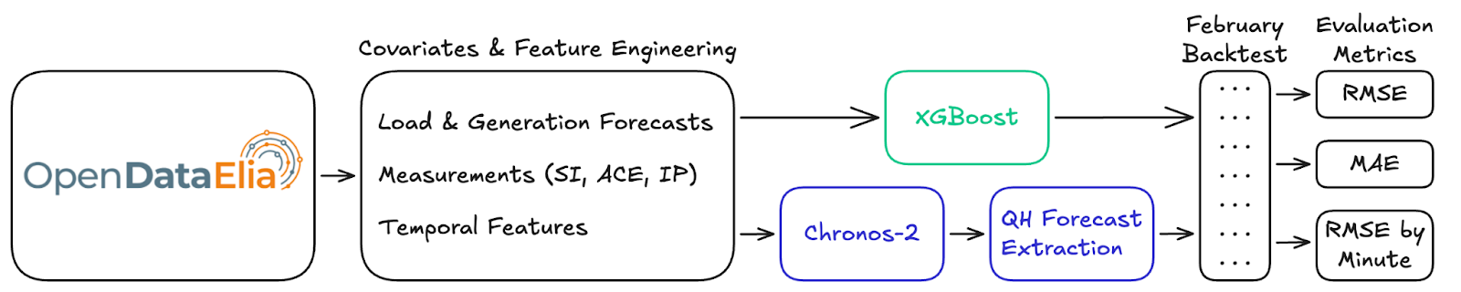
Figure 4: Forecasting pipeline for evaluating XGBoost and Chronos-2, from data ingestion and feature engineering to backtesting and performance metrics.
Applying Chronos-2 in this setting requires additional adaptations. The model is used in a zero-shot configuration with a long historical context (2048 timesteps) and a 15-minute prediction horizon, aligned with the operational forecasting task.
As discussed before, the challenge lies in defining the forecasting target itself. The quantity of interest is the quarter-hour SI, which is:
- A cumulative average over a 15-minute interval
- Only published at the end of that interval
- Constant within each quarter-hour once known
This makes it unsuitable as a direct training target in a rolling forecasting setup, as it would introduce leakage within the quarter-hour.
To address this, we reformulate the problem at minute resolution:
- The target becomes the cumulative minute-level SI
- It produces a 15-minute ahead forecast
- The prediction corresponding to the last minute of the quarter-hour is used as a proxy for the QH SI.
This approach ensures that the target remains causal while still aligning with the operational objective. Effectively, the model learns to anticipate how the cumulative imbalance will evolve over the remainder of the quarter-hour, using only information available at prediction time. A visualization of how these forecasts are extracted can be seen in Figure 5.
Together, these adjustments ensure that both models operate under identical, realistic constraints, and highlight an important practical insight: even for foundation models, careful problem formulation and data alignment remain critical for real-world deployment.
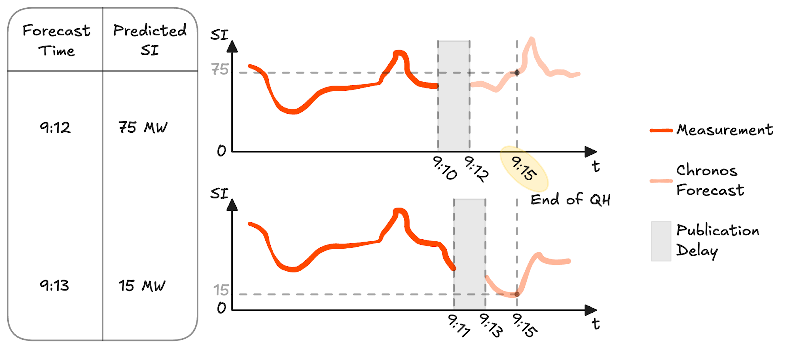
Figure 5: Illustration of how QH SI forecasts are extracted in a rolling backtest. At each minute, predictions are generated using only information available up to the publication delay, and the forecast corresponding to the final minute of the quarter-hour is used as the QH SI estimate.
Results & Practical Evaluation: From Performance to Production
Forecasting Performance
Figure 6 shows the quantitative comparison of Chronos-2 against two benchmarks: a tuned XGBoost model and a naive persistence baseline.
In terms of aggregate performance, the XGBoost model achieves the strongest results (RMSE 59.38, MAE 38.16). Chronos-2 follows with an RMSE of 66.34 and MAE of 44.43, clearly outperforming the persistence baseline (RMSE 77.67, MAE 51.61).
Looking at performance within each quarter-hour in Figure 7, all models exhibit higher errors at the beginning of the interval and improve as more information becomes available. Chronos-2 follows this pattern closely and remains competitive throughout, although it does not surpass the XGBoost model
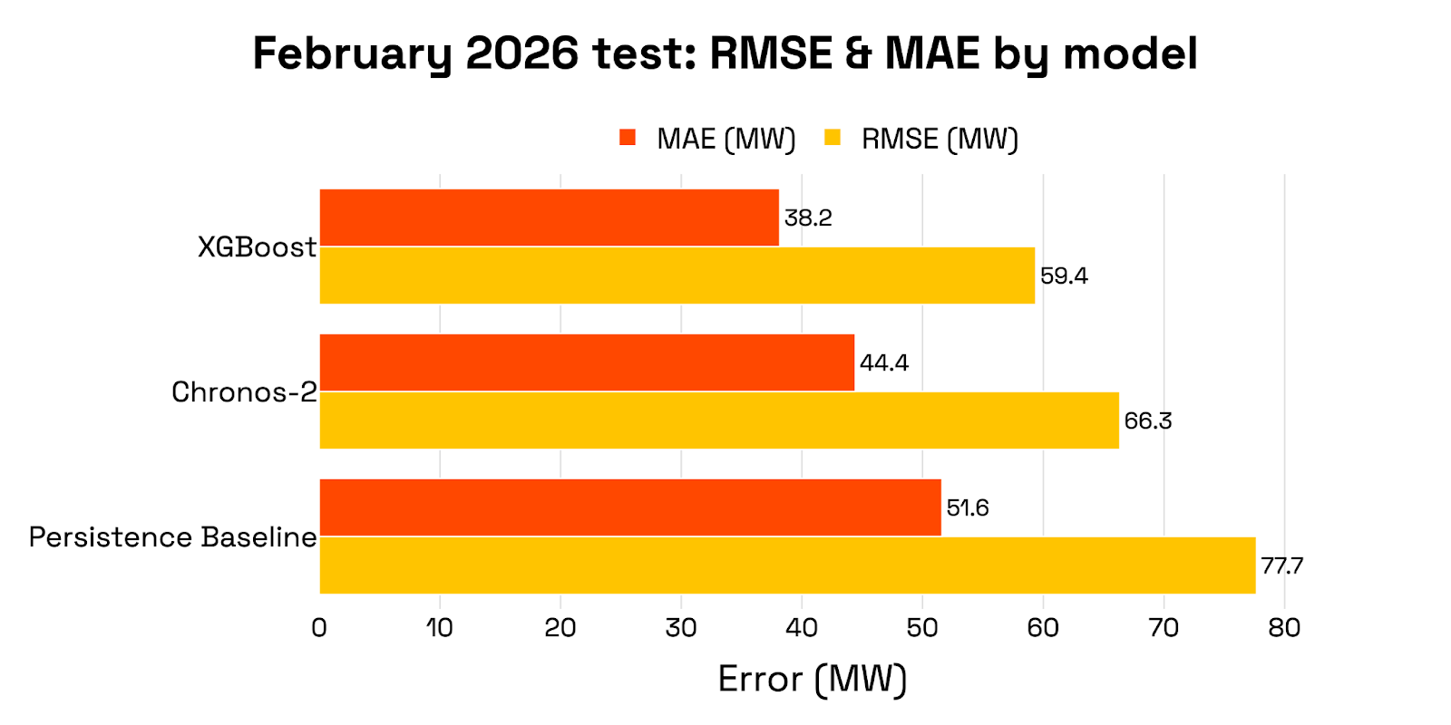
Figure 6: Performance metrics of Chronos-2, XGBoost and the persistence baseline model. Lower values indicate better performance. RMSE penalizes larger errors more strongly, while MAE reflects the average magnitude of errors.
 Figure 7: Intra-QH RMSE as a function of the minute within the QH. Forecast accuracy improves over time, with Chronos-2 and XGBoost outperforming the persistence baseline throughout the interval.
Key Takeaways
While Chronos-2 delivers solid out-of-the-box performance, it does not yet outperform a well-engineered production model. This is not entirely surprising: SI forecasting is a non-standard problem, with a cumulative quarter-hour target and strict data availability constraints that make it inherently challenging.
At the same time, Chronos-2 requires no training or fine-tuning and performs significantly better than the simple baseline. This positions it as a strong baseline model that can be deployed quickly.
These results also highlight the strong potential of TSFMs. Given the rapid pace of progress in this space, it is plausible that future iterations, or modest adaptations, will further close the gap with specialized models.
Beyond predictive performance, validation proved to be a significant challenge in practice. Backtesting was computationally expensive and time-consuming. Due to the problem formulation, each minute requires generating multiple forecasts and selecting the one corresponding to the end of the quarter-hour. Combined with a relatively high inference time per forecast, this resulted in long evaluation cycles: running a single month of data took several days in a containerized setup, making rapid iteration difficult.
Finally, the infrastructure overhead is less a property of the model itself and more a function of the operational requirements: forecast frequency, robustness expectations (e.g. retries, fallbacks), and system design choices. While foundation models reduce modeling effort, they do not eliminate the need for carefully engineered pipelines to handle throughput, reliability, and integration into existing systems. This reinforces a key insight: foundation models are not yet plug-and-play solutions. Their successful application still depends on careful problem formulation, data alignment, and integration into real-world systems.
Final Verdict
Chronos-2 shows that TSFMs can already deliver strong out-of-the-box performance, making them attractive as fast-to-deploy baseline models.
However, they do not yet outperform well-engineered production systems, and their practical adoption comes with non-trivial challenges in validation, scalability, and integration. TSFMs are therefore best seen not as replacements for specialized models, but as powerful starting points, particularly valuable when speed is prioritized over maximum performance and reliability.
At ML6, we see their role as part of a broader forecasting stack, where combining domain knowledge with the right modeling approach remains key to delivering real impact.
If you are looking to build a production-grade forecasting pipeline or evaluate the role of foundation models in your operations, get in touch with ML6 to leverage state-of-the-art expertise tailored to your specific context.