Why care about dynamic pricing?
Dynamic pricing aims to actively adapt product prices based on insights about customer behavior.
This pricing strategy has proven exceptionally effective in a wide range of industries: from e-commerce (e.g., TB International) to sports (e.g., Ticketmaster) and from food delivery (e.g., GO-JEK) to automotive (e.g., Carro) as it allows to adjust prices to changes in demand patterns.
It is hardly surprising that recent times of extraordinary uncertainty and volatility caused a surge in the adoption of dynamic pricing strategies with an estimated 21% of e-commerce businesses reportedly already using dynamic pricing and an additional 15% planning to adopt the strategy in the upcoming year.
To find a big success story, we should look no further than Amazon who (on average) change their products’ prices once every 10 minutes. They attribute roughly 25% of their e-commerce profits to their pricing strategy.
In what follows we’ll take a practical look at the working principles & challenges in the field of dynamic pricing, followed by some final considerations.
Back to basics
The beginning is usually a good place to start so we’ll kick things off there.
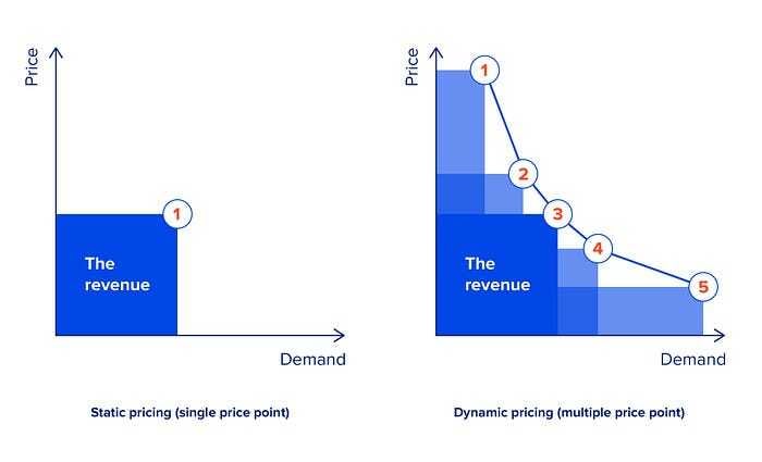
The one crucial piece of information we need in order to find the optimal price is how demand behaves over different price points.
If we can make a decent guess of what we can expect demand to be for a wide range of prices, we can figure out which price optimizes our target (i.e., revenue, profit, …).
For the keen economists amongst you, this is beginning to sound a lot like a demand curve.
Estimating a demand curve, sounds easy enough right?
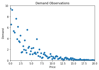
Let’s assume we have demand with constant price elasticity; so a certain percent change in price will cause a constant percent change in demand, independent of the price level. In economics, this is often used as a proxy for demand curves in the wild.
So our demand data looks something like this:
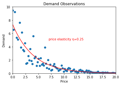
Alright now we can get out our trusted regression toolbox and fit a nice curve through the data because we know that our constant-elasticity demand function has this form:
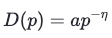
with shape parameter a and price elasticity η
Now that we have a reasonable estimate of our demand function, we can derive our expected profit at different price points because we know the following holds:
Note that fixed costs (e.g., rent, insurance, etc.), per definition, don’t vary when demand or price changes. Therefore, fixed costs have no influence on the behavior of dynamic pricing algorithms.
Finally, we can dust off our good old high-school math book and find the price which we expect will optimize profit which was ultimately the goal of all this.
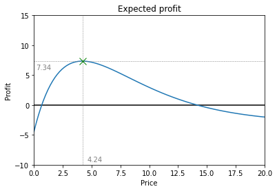
Voilà there you have it: we should price this product at 4.24 and we can expect a bottom-line profit of 7.34
So can we kick back & relax now? Well, there are a few issues with what we just did.
The demands they are a-changin’
We arrive at our first bit of bad news: unfortunately, you can’t just estimate a demand curve once and be done with it.
Why? Because demand is influenced by many factors (e.g., market trends, competitor actions, human behavior, etc.) that tend to change a lot over time.
Below you can see an (exaggerated) example of what we’re talking about:
Now, you may think we can solve this issue by periodically re-estimating the demand curve.
And you would be very right! But also very wrong as this leads us nicely to the next issue.
Where are we getting this data anyways?
So far, we have assumed that we get (and keep getting) data on demand levels at different price points.
Not only is this assumption unrealistic, but it is also very undesirable
Why? Because getting demand data on a wide spectrum of price points implies that we are spending a significant amount of time setting prices that are either too high or too low!
Which is ironically exactly the opposite of what we set out to achieve.
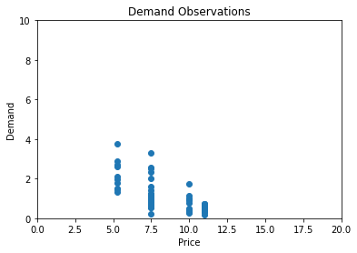
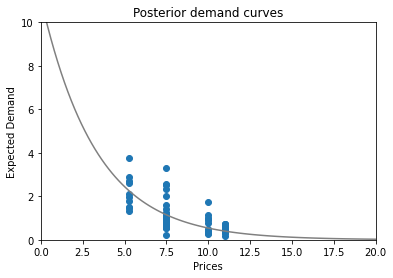
In practice, our demand observations will rather look something like this:
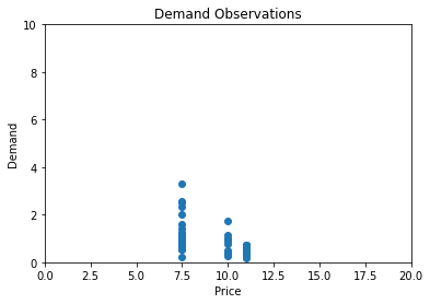
As we can see, we have tried three price points in the past (€7.5, €10 and €11) and collected demand data.
On a side note: keep in mind that we still assume the same latent demand curve and optimal price point of €4.24
So (for the sake of the example) we have been massively overpricing our product in the past.
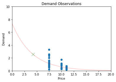
This limited data brings along a major challenge in estimating the demand curve though.
Intuitively, it makes sense that we can make a reasonable estimate of expected demand at €8 or €9, given the observed demand at €7.5 and €10.
But can we extrapolate further to €2 or €20 with the same reasonable confidence? Probably not.
This is a nice example of a very well-known problem in statistics called the “exploration-exploitation trade-off”
Exploration: We want to explore the demand for a diverse enough range of price points so that we can accurately estimate our demand curve.
Exploitation: We want to exploit all the knowledge we have gained through exploring and actually do what we set out to do: set our price at an optimal level.
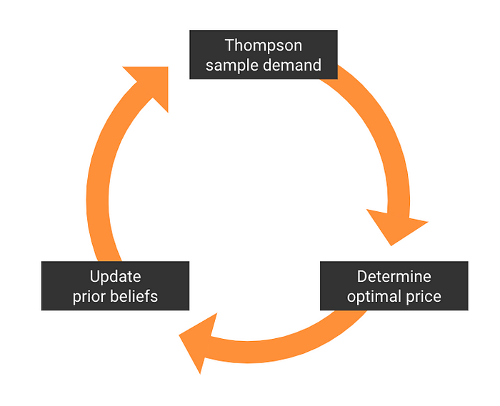
Enter: Thompson Sampling
As we mentioned, this is a well-known problem in statistics. So luckily for us, there is a pretty neat solution in the form of Thompson sampling!
Basically, instead of estimating one demand function based on the data available to us, we will estimate a probability distribution of demand functions or simply put, for every possible demand function that fits our functional form (i.e. constant elasticity) we will estimate the probability that it is the correct one, given our data.
Or mathematically speaking, we will place a prior distribution on the parameters that define our demand function and update these priors to posterior distributions via Bayes’ rule, thus obtaining a posterior distribution for our demand function
Thompson sampling then entails just sampling a demand function out of this distribution, calculating the optimal price given this demand function, observing demand for this new price point and using this information to refine our demand function estimates.
So:
- When we are less certain of our estimates, we will sample more diverse demand functions, which means that we will also explore more diverse price points. Thus, we will explore.
- When we are more certain of our estimates, we will sample a demand function close to the real one & set a price close to the optimal price more often. Thus, we will exploit.
With that said, we’ll take another look at our constrained data and see whether Thompson sampling gets us any closer to the optimal price of €4.24.
Let’s start working our mathemagic:
We’ll start off by placing semi-informed priors on the parameters that make up our demand function.
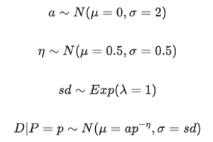
These priors are semi-informed because we have the prior knowledge that price elasticity is most likely between 0 and 1. As for the other parameters, we have little knowledge about them so we can place a pretty uninformative prior.
If that made sense to you, great. If it didn’t, don’t worry about it
Now that our priors are taken care of, we can update these beliefs by incorporating the data at the €7.5, €10 and €11 price levels we have available to us.
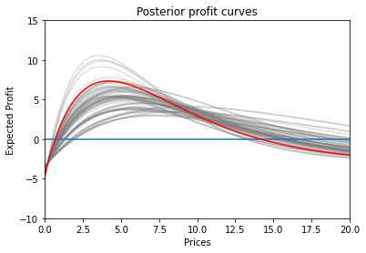
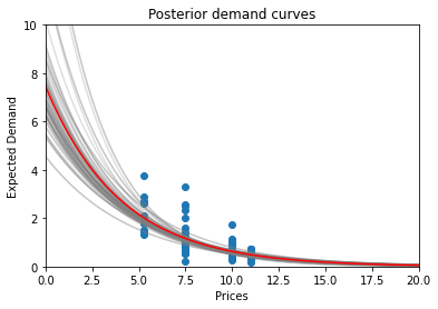
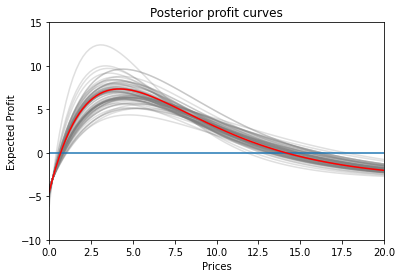
The resulting demand & profit curve distributions look a little something like this:
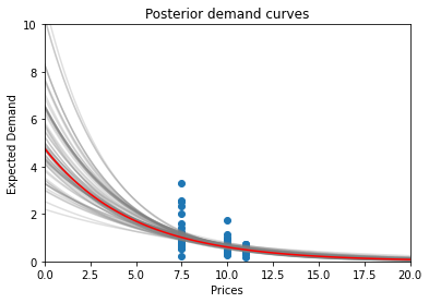
It’s time to sample one demand curve out of this posterior distribution.
The lucky curve is:
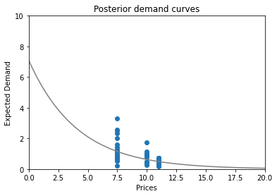
This results in the following expected profit curve
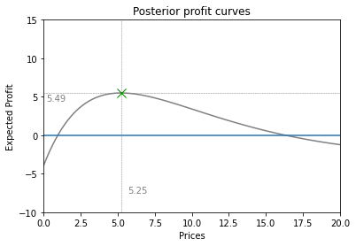
And eventually, we arrive at a new price: €5.25! Which is indeed considerably closer to the actual optimal price of €4.24
Now that we have our first updated price point, why stop there?
With “pure” Thompson sampling, we would sample a new demand curve (and thus price point) out of the posterior distribution every time. But since we are mainly interested in seeing the convergence behavior of Thompson sampling, let’s simulate 10 demand points at this fixed €5.25 price point.
We know the drill by now.
Let’s recalculate our posteriors with this extra information.
We immediately notice that the demand (and profit) posteriors are much less spread apart this time around which implies that we are more confident in our predictions.
Now, we can sample just one curve from the distribution.
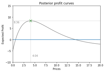
And finally, we arrive at a price point of €4.04 which is eerily close to the actual optimum of €4.24
Some things to think about
Because we have purposefully kept the example above quite simple, you may still be wondering what happens when added complexities show up.
Let’s discuss some of those concerns FAQ-style:
Isn’t this constant-elasticity model a bit too simple to work in practice?
Brief answer: usually yes it is.
Luckily, more flexible methods exist.
We would recommend using Gaussian Processes. We won’t go into how these work here but the main idea is that it doesn’t impose a restrictive functional form onto the demand function but rather lets the data speak for itself.
If you do want to learn more, we recommend these links: 1, 2, 3
Price optimization is much more complex than just optimizing a simple profit function?
It sure is. In reality, there are many added complexities that come into play, such as inventory/capacity constraints, complex cost structures, …
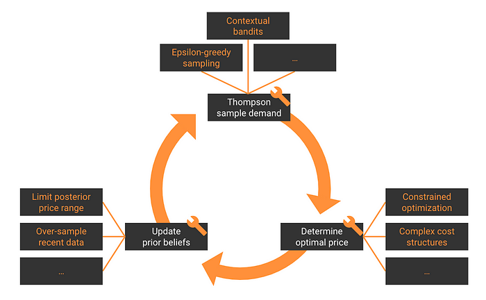
The nice thing about our setup is that it consists of three components that you can change pretty much independently from each other.
This means that you can make the price optimization pillar arbitrarily custom/complex. As long as it takes in a demand function and spits out a price.
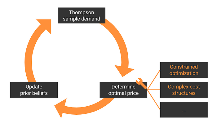
You can tune the other two steps as much as you like too.
Changing prices has a huge impact. How can I mitigate this during experimentation?
There are a few things we can do to minimize risk:
- A/B testing: You can do a gradual roll-out of the new pricing system where a small (but increasing) percentage of your transactions are based on this new system. This allows you to start small & track/grow the impact over time.
- Limit products: Similarly to A/B testing, you can also segment on the product-level. For instance, you can start gradually rolling out dynamic pricing for one product type and extend this over time.
- Bound price range: Theoretically, Thompson sampling in its purest form can lead to any arbitrary price point (albeit with an increasingly low probability). In order to limit the risk here, you can simply place an upper/lower bound on the price range you are comfortable experimenting in.
On top of all this, Bayesian methods (by design) explicitly quantify uncertainty. This allows you to have a very concrete view of the demand estimates’ variance
What if I have multiple products that can cannibalize each other?
Here it really depends
- If you have a handful of products, we can simply reformulate our objective while keeping our methods analogous.
Instead of tuning one price to optimize profit for the demand function of one product, we tune N prices to optimize profit for the joint demand function of N products. This joint demand function can then account for correlations in demand within products. - If you have hundreds, thousands or more products, we’re sure you can imagine that the procedure described above becomes increasingly infeasible.
A practical alternative is to group substitutable products into “baskets” and define the “price of the basket” as the average price of all products in the basket.
If we assume that the products in baskets are substitutable but the products in different baskets are not, we can optimize basket prices independently from one another.
Finally, if we also assume that cannibalization remains constant if the ratio of prices remains constant, we can calculate individual product prices as a fixed ratio of its basket price.
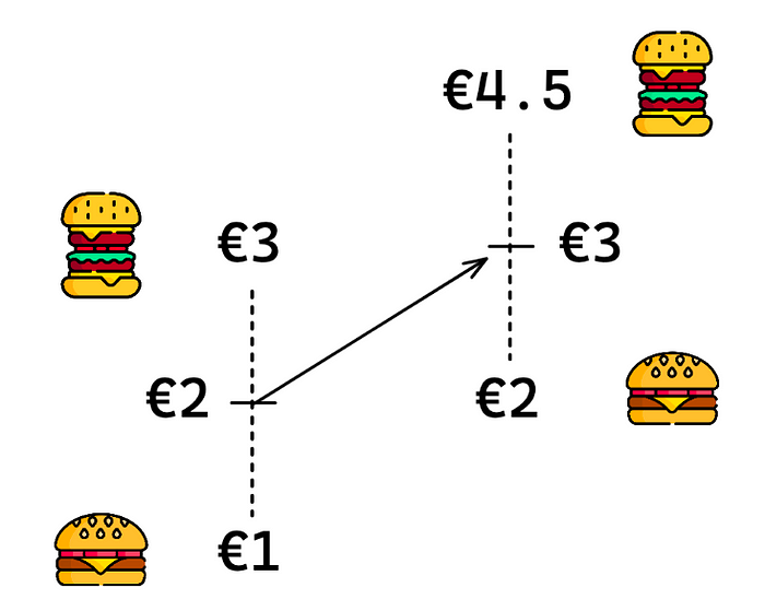
For example, if a “burger basket” consists of a hamburger (€1) and a cheeseburger (€3), then the “burger price” is ((€1 + €3) / 2 =) €2. So a hamburger costs 50% of the burger price and a cheeseburger costs 150% of the burger price.
If we change the burger’s price to €3, a hamburger will cost (50% * €3 =) €1.5 and a cheeseburger will cost (150% * €3 =) €4.5 because we assume that the cannibalization effect between hamburgers & cheeseburgers is the same when hamburgers cost €1 & cheeseburgers cost €3 and when hamburgers cost €1.5 & cheeseburgers cost €4.5
Is dynamic pricing even relevant for slow-selling products?
The boring answer is that it depends. It depends on how dynamic the market is, the quality of the prior information, …
But obviously, this isn’t very helpful.
In general, we notice that you can already get quite far with limited data, especially if you have an accurate prior belief on how the demand likely behaves.
For reference, in our simple example where we showed a Thompson sampling update, we were already able to gain a lot of confidence in our estimates with just 10 extra demand observations.
Demo time
Now that we have covered the theory, you can go ahead and try it out for yourself!
You can access our interactive demo here: https://huggingface.co/spaces/ml6team/dynamic-pricing